My take on data quality: Tier 2

Preserving data quality: pipeline lags, schema breakage, self-healing

In the previous post (“My take on data quality: whitelist approach, correct by design”) we looked at data quality through the lens of minimal independent data elements: anchors, attributes and links. We discussed the first tier: how to establish the input data quality for a specific query.

Let’s continue with the second tier: maintaining data elements, so that they stay up-to-date without losing quality. (2700 words)

Basically, we need to talk about pipelines, but our approach to organizing pipelines is different: each pipeline handles only a single data element: anchor (list of IDs), attribute (ID + value), and link (ID + ID). Entangling several data elements in a single pipeline introduces complexity and increases the risk of losing data quality, which is our focus.

This text is completely database-agnostic, we won’t mention any tool names.

Attribute pipeline

So, suppose that we have an Item anchor and an attribute that contains an SKU of that item. In the first part we defined an SQL query that selects the current version of the dataset:

SELECT item_id, sku
FROM items
WHERE sku IS NOT NULL AND sku <> ‘‘;

We query the “items” table, stored in our primary database; there are other columns in it, but we ignore them here. We skip the rows that contain NULL or empty values, because we want only the clean data.

We keep the result of the query in a table called “items__sku” (double underscore) in our data warehouse. We want to keep this table up-to-date.

Our concerns are two-fold: timing and correctness. As for timing, we’ll discuss:

• the idea of pipeline lags;

• three scenarios of lagging pipeline:

  • starting delay;

  • processing delay;

  • processing failure and restarts;

• treating schema issues as lagging;

• recovering from outages longer than a single cycle;

• handling empty cycles when no data changes happen.

Pipeline lags

First thing we must say is that this table is always lagging relative to the primary database. Even if we use real-time data streaming, there is always a lag. If we use more common batch updates (every 24 hours, every hour, and so on) — we have a lag.

Second, we need to monitor this lag so that we could alert when the lag becomes unacceptable (actually, even before that).

We need to carefully define lag, because there are some scenarios where naive definitions break.

One interesting thing here is that we treat schema issues using the same lag framework.

Let’s take a low-frequency batch processing, such as 24 hours. We’ll see that the general approach is valid for all durations, even for real-time processing.

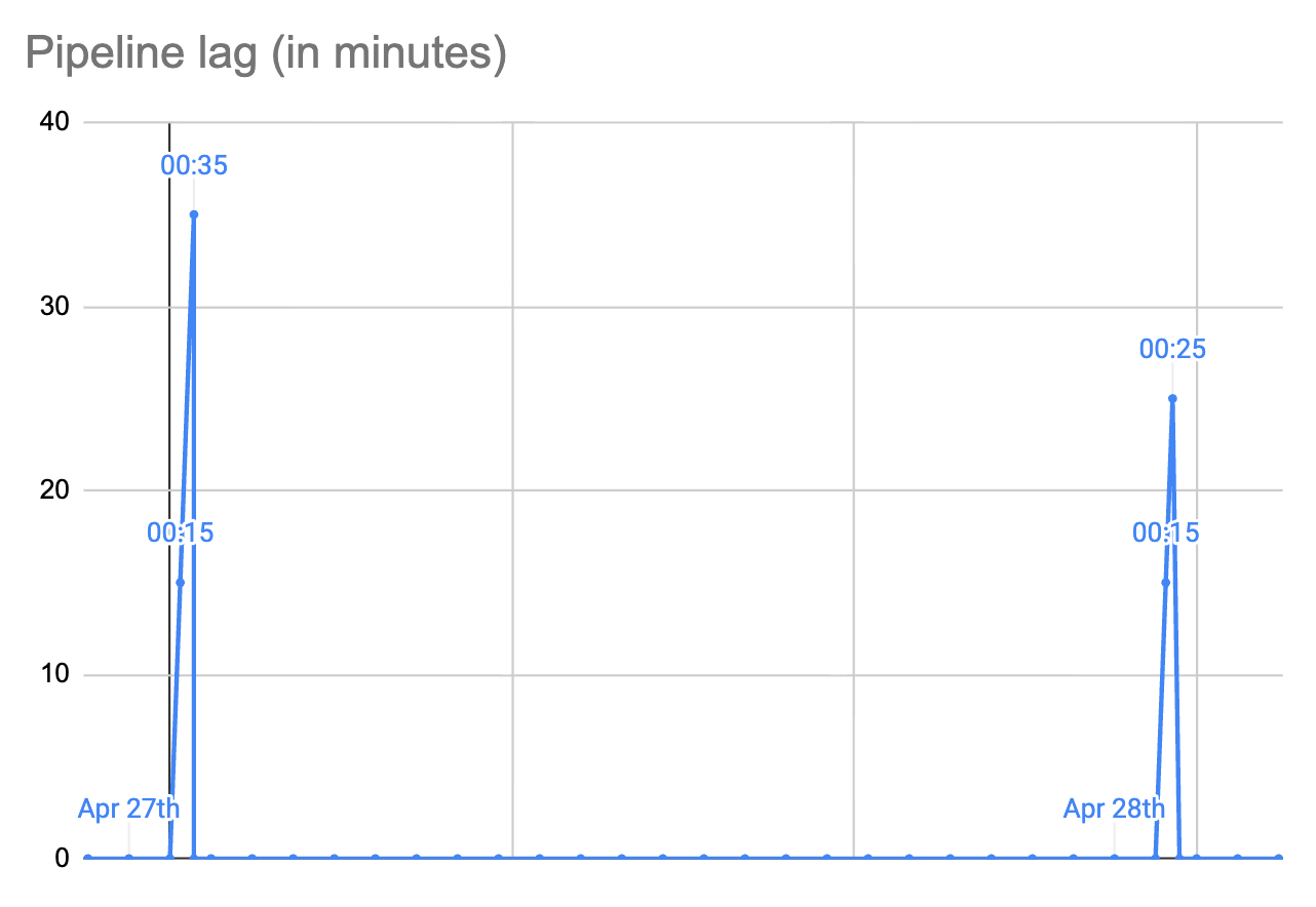
Here is the happy path:

• Mon, April 27th, 00:00:00: our system works, updating the “items” table variously: inserting new rows, updating some SKUs to valid values, or to sentinel values such as NULL or empty string.

• Tue, April 28th, 00:00:00: a processing pipeline starts, maybe not immediately. Its goal is to process all changes that happened during April 27th, and to update the “items__sku” table accordingly;

• 00:15:00: the pipeline starts around that time, and it’s expected to run for around 15 minutes.

• 00:35:00: the pipeline finishes (it was delayed a bit, and it took a few minutes more than expected, that’s fine).

• 00:35:01: The main system proceeds as usual, updating the “items” table.

• Wed, April 29th, 00:00:00: next iteration starts.

What is the lag here?

• on Tuesday, at 00:00:00, lag is 0 seconds, it starts to grow;

• at 00:15:00 the lag is 900 seconds (15 * 60);

• at 00:34:59 the lag is 2099 seconds (34 * 60 + 59);

• at 00:35:00 the processing job finishes successfully, and the lag is reset to 0;

• the lag stays at 0 until the end of the day, and it will start growing again at Wednesday midnight;

So, we have a sawtooth graph here.

The daily processing is expected to finish within an hour (maximum lag: 3600 seconds), and if it takes more than that we need to start alerting.

How did we arrive at that “an hour” estimate? We looked at the typical processing time, and we agreed with our customers that one hour is fine. In our example above, all went well.

Simple causes of lag

What could go wrong here, and how would it affect the lag?

Case 1: starting delay. Suppose that the cluster is overloaded and our processing job is not scheduled for a long time. For example, it starts at 01:10:00 (lag: 4200 seconds). It runs for 15 minutes, as expected, and ends successfully at 01:25:00 (lag: 5100 seconds).

We’ll get an alert at 01:00:00, but it will resolve itself in 25 minutes. Maybe we’ll help it by freeing up some cluster resources, too.

Case 2: processing delay. Another possibility is that the processing job is started normally, but would run longer than expected. Example: start at 00:15:00, successfully ends at 01:15:00 (lag: 4500 seconds).

Same here, we’ll get an alert at 01:00:00, but it will resolve itself in 15 minutes. We may help.

Case 3: processing failure. The job starts normally, but for some reason fails after 5 minutes. Maybe it’s killed to free up resources, or there is an intermittent node failure. Normally, the cluster will restart the job quickly, and hopefully it will run to the end.

Maybe it will even fit into the accepted lag threshold. Maybe it will be restarted several times, but will eventually finish successfully. Maybe it would need the operator’s help.

Treating schema issues as lagging

Case 4: incompatible schema changes. Suppose that somebody renamed or dropped the “items” table, or the “sku” column. In other words, the upstream schema was changed without our knowledge, and it breaks our pipeline.

The processing job starts, tries to execute some SQL, gets a server error, and terminates abnormally. The scheduler restarts it, it quickly fails again, and so on.

We can detect and treat this in mostly the same way as other failures. At 01:00:00 we start getting an alert and decide what to do: maybe ask the upstream to fix their database, or change the query because the column is now in a different place.

We can make it better if we are able to distinguish between transient and permanent job failures. When the job starts failing for a “permanent” reason (such as SQL query error), we can trigger alerting earlier, so that we have more time for fixes.

This is basically a normal SRE (software reliability engineering) practice, applied to data processing pipelines.

I see lots of complaints from people who have to work in non-cooperating environments. They experience schema changes, and their data silently stops processing until somebody notices. The approach explained here allows to handle schema breakage more proactively.

Longer outages

Failures discussed above were resolved within 24 hours in our examples above. But what if we have a longer outage? Naive handling of this case may lead to the system’s inability to recover on its own.

Note that this is also applicable to other frequencies. If you have an hourly job, you already need to think how your system will handle an outage that lasts for several hours. If you are not careful here, the system may not self-heal and will demand more manual work, further increasing lag.

Suppose that the main system runs normally, generating data changes, but our pipeline processing cluster experienced a prolonged outage, lasting, say 72 hours.

Suppose that the last successfully processed day was April 27th (it happened before 01:00:00 on 28th). Our cluster went into a death spiral, and it only recovered on May 1st.

Our job needs to process three days worth of data: 28th, 29th, and 30th of April. It is now the early hours of May 1st.

The lag is horrible: 50+ hours, but the cluster schedules a new job. What does it do?

One thing that it could do is to try and catch up the entire time period, which is 3x the usual amount. This may or may not work, depending on how the job is written. This can easily lead to a greater chance of failure.

Time right after the outage is a very bad time to have a greater chance of failure. The rest of the system, all other pipelines, are also recovering. If they all are written in the same way, there is a chance that the system will go into a death spiral (again) because everything runs on overdrive.

A way to handle this is to sequentially process each day separately.

• The job runs, sees that it’s supposed to process 3 days, but it only processes data changed on 28th of April.

• When that day is processed, the day is marked as done, so that the lag now decreases from 50 hours to 26+ hours.

• The same or a different job runs, and processes data changed on 29th. The lag decreases from 26+ hours to 2+ hours.

• Finally, data from April 30th is processed, and the lag becomes 0.

The goal of this is to make incremental progress. If you run all three days at the same time, and the job fails, there is no visible progress.

Empty cycle

Another important case that we must consider is what to do if there were no changes in a certain cycle.

Suppose that there were no new items and no SKU changes in the entire 24 hours. Our processing job runs, sees that there is nothing to do, so it does nothing. But it must signal somehow that it has actually run successfully.

If your monitoring system uses a condition like “when was the most recent change” just looking at data itself, it will think that there is a 24 hour lag, which would be a bug.

You need a separate place where you keep the information about the most recently processed period of time. Two columns are enough: say, the name of the destination table (“items__sku”), and the last successfully processed date (“2026-04-28”).

Note that logically, this is not a timestamp, it’s an indicator of the last successfully processed period (e.g., “2026-04-28”). For hourly jobs it’s going to be, e.g. “2026-04-28 17:00”. It can be implemented as a timestamp, but you need to think about what happens during DST changes.

Correctness of data

The easiest way to keep “items__sku” up-to-date is to just execute the SQL query, fetch all the data into a new table, and then rename. This is an extremely simple method that has a very low risk of messing with the data correctness. Unfortunately, it quickly becomes infeasible if the dataset is big enough.

Because of that, we need to make incremental data updates.

1/ New rows in “items”, created during the processing window, need to be inserted into “items__sku” (only those that have valid values).

2/ SKU values changed during the processing window need to be updated (if old and new values are valid).

3/ SKU values that changed from empty to a valid value, need to be inserted.

4/ SKU values that changed from a valid value to an empty value need to be deleted.

5/ For rows that were deleted from “items”, the corresponding rows in “items__sku” need to be deleted.

It’s easy to overlook one or more of the cases listed here. That would cause data discrepancies between “items” and “items__sku”.

It’s easier to think about data correctness here because we think in terms of minimal attribute tables such as “items__sku”; same for anchor tables and link tables, discussed below.

Here, I’m pretty sure that only the five scenarios above are possible. Testing your change processing code thus requires only a very small amount of test cases.

Checking correctness

No matter how correct your change processing code is, you need to continuously monitor data correctness between the source and destination tables.

1/ First, you make a snapshot of both tables. This would probably be the trickiest part, depending on the size of the dataset. Various databases provide different options. The idea is to reduce the amount of changes in flight as much as possible.

Sometimes it may be unfeasible; in that case you would always have some discrepancies. You need to find a way to distinguish between temporary and permanent discrepancies. For example, you can run the cross-checking two times and see which of the earlier discrepancies went away and which remained.

2/ Second, you run the entire SQL query from the source snapshot table, and generate a clean new destination table.

3/ Third, you compare the normal destination table with the clean one, and analyze discrepancies looking at the data.

4/ Based on that, you hopefully find problems in your change processing code and fix them. Maybe you forgot about one of the five scenarios listed above. Maybe your pipeline does not handle outages properly. Maybe your source table does not report data changes properly: for example, it’s not updating timestamps that you rely upon.

5/ After that, you need to re-sync the entire dataset into the destination table.

This cross-check process needs to run regularly, but not as often as the normal cadence. Say, for the daily processing job you need to run cross-checking maybe every two weeks.

The important thing here is that this process of fixing the code needs to move towards converging. It’s fine to have discrepancies initially, but after a number of iterations discrepancies must be an exception, and not the norm. In other words, you need to prevent regressions.

I see lots of people complaining that their system “constantly breaks”: it should be possible to build a system that does not break constantly. This topic belongs to the discussion of Tier 3, which we’ll talk about in the next post.

SQL query changes

Sometimes you find out that the underlying SQL query needs to be fixed. For example, you may need to add another sentinel value (“UNKNOWN”):

SELECT item_id, sku
FROM items
WHERE sku IS NOT NULL AND sku <> ‘‘ AND sku <> ‘UNKNOWN’;

There are some rows in “items__sku” that contain this value: “UNKNOWN”. From now on, those values would be skipped automatically, because that’s how the normal pipeline runs. But you would also expect the older values to disappear.

Thankfully, this can be done by just running the same re-sync process that you run when the discrepancies are detected.

Re-sync implementation

In the text above, we mentioned three scenarios of data sync between the source table (“items”) and destination table (“items__sku”):

• initial data copy into an empty destination table;

• re-sync after discrepancies were detected and the incremental processing has been fixed;

• re-sync after the data filtering SQL is changed;

The good news is that all three scenarios could be handled by exactly the same code. To reduce the chance of mistakes, this should be handled by the exact same code.

This post is getting quite long. We still need to cover a few more technical aspects, such as a) anchor pipelines and link pipelines; b) using timestamps to reliably detect changes; c) generating more familiar representations without losing quality. That’s a topic for one more extra post, because I’d like to start working on Tier 3 discussion.

Conclusion

In the previous post we’ve discussed Tier 1. We used the whitelist approach to establish quality data elements: anchors, attributes, and links. Each element has a corresponding SQL query, or something similar.

In this post we started discussing Tier 2. Every concern discussed in this text is aimed at the single goal: to reduce the risk that your destination table diverges from the source dataset. When the pipeline lag is zero you want a guarantee that the data is correct. When the pipeline lag is non-zero you want to be sure that your monitoring will tell you about that so that you can make interventions if needed.

One uncommon aspect of our approach is that we treat upstream schema changes that break our pipeline as a sub-case of processing delay. We detect it using the same monitoring and alerting infrastructure that we use for the usual variability of data processing time.

In the classic system design maxim: “Make It Work, Make It Right, Make It Fast”, we are firmly in the “Make It Right” position.

In the next post we’ll discuss Tier 3: keeping the entire data warehouse up to date. We’ll focus more on the aspects of system management:

• how to react to outages;

• how to handle changes in the source database;

• how to manage consumers that depend on our data;

Stay tuned!